
Representing a Toroidal Grid
When I first proposed Mazes for Programmers @amazon | @b&n, my original outline was enormous. It was going to be the de-facto reference for all things related to maze algorithms. I think I estimated the length of the book–when finished–to be somewhere in the neighborhood of 500 pages.
I went into this with big dreams. Among many other things (some of which I may blog about eventually), I was going to have a chapter that went into detail about how to map a grid onto three-dimensional objects like spheres, cubes, toruses, and so forth.
After my proposal was accepted and I got down to business, my editor (Jackie Carter) talked me down to a more reasonable 250-300 pages, which could only be done if I sacrified a significant portion of my outline. A lot of things got cut. I managed to keep the bit about spheres, cubes, and even Möbius strips, but (alas!) the toruses didn’t quite make the grade.
This is what blogs are for, I guess! I’d like to make up for that shattered dream of mine and share a bit about how I would represent a grid that can be mapped onto a torus with a minimum of distortion. (A torus, you’ll recall, is a donut shape–a tube that connects to itself and forms a circle.)
Now, you could simply take a rectangular grid of cells and map it onto a torus, like wallpapering a donut. The problem with that approach is that you’re going to wind up with a distorted grid.
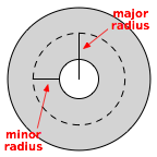
Consider. A torus, viewed from above, is essentially two concentric circles:
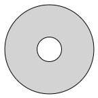
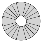
Simple geometry–or even intuition–will tell you that the inner of those two circles has a smaller circumference than the outer circle. If you were to apply a 10x10 grid to such a torus, the ten cells on the interior circumference would be smaller than those on the outer circumference. We can show this distortion simply by drawing radial lines between the two circles. See how they are further apart on the outside, than on the inside?
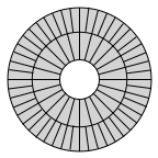
Now, if you make the torus thin enough, the difference between the circumferences becomes smaller, which means the distortion grows less. You can also reduce the distoration by dividing the grid into more cells. But, really, these are very specific solutions to the problem. For a more general solution, we can instead employ adaptive subdivision to split cells in half when they begin to distort beyond some threshold.
(This is the same thing I talk about on page 103 of my book.)
Toroidal grids share a lot with spherical grids (pg. 238 of my book), so some of this may sound very familiar if you’ve been through that. A spherical grid is basically a soup-can wrapper rolled so the east and west edges touch (and then with a bit of magic applied to the north and south edges so they reduce to a point). The same is true of a torus, but with another interesting difference. Picture that soup can wrapper. Now, roll it so that the north and south boundaries touch. Then, taking that cylindrical tube, bend it around donut-style, so that the east and west boundaries touch.
See that? Toroidal grids wrap in both dimensions!
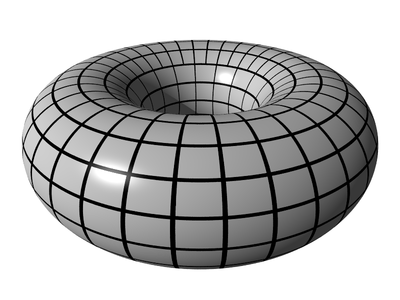
Just as I did in my book when dealing with spheres, we’re going to tackle this as simply as possible. We’ll just create a grid that wraps in both dimensions, and then map it onto the 3D geometry of a torus using POV-Ray. That is to say, our final result will look like this:
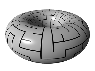
We aren’t going to be generating actual geometry for the walls, here. (Though, that’s a lot of fun, too! Maybe I’ll talk about that in another article…)
Got all that? Let’s do it. We’ll create an adaptively subdivided, toroidal grid of cells.
Implementation
I’ll use Ruby for my implementation, but the underlying ideas ought to map very cleanly to whatever language you’re using. Also, while I’m not using any of the code from my book here, you could easily use the code from there to do this exercise, if you’d prefer.
We’ll start by implementing a simple Cell class. It will need to:
- hold references to its neighbors to the west and east (clockwise and counterclockwise around the torus).
- hold references to its neighbors to the north and south (moving poloidally around the torus). Because we’ll be adaptively subdividing the grid, a cell may have more than one neighbor in each of those directions!
- indicate that a passage has linked it with a neighboring cell.
Here’s what I’ve got:
class Cell
  attr_reader :row, :column
  attr_reader :north, :south
  attr_accessor :east, :west

  def initialize(row, column)
    @row, @column = row, column
    @north, @south = [], []
    @east = @west = nil
    @links = {}
  end

  def neighbors
    [ east, west, *north, *south ].compact
  end

  def link!(neighbor, once=false)
    @links[neighbor] = true
    neighbor.link!(self, true) unless once
  end

  def linked?(neighbor)
    @links[neighbor]
  end

  def links
    @links.keys
  end
end
The grid, then, will be a collection of these cells, arranged very particularly.
We’ll call our grid ToroidalGrid:
class ToroidalGrid
end
It will represent a unit torus–that is, a torus with a major radius of 1.
We’ll initialize it by telling it how many rows we want in our grid (must be at least three, mostly for esthetic reasons), as well as what the minor radius is. (Because the major radius is always going to be 1, the minor radius will necessarily be a value between 0 and 1.)
attr_reader :row_count, :minor_radius

def initialize(row_count, minor_radius)
  if row_count < 3
    raise ArgumentError, "must have at least 3 rows"
  end

  if minor_radius <= 0 || minor_radius >= 1
    raise ArgumentError, "minor radius must be in (0,1)"
  end

  @row_count = row_count
  @minor_radius = minor_radius

  configure_grid!
end
The magic math happens in the configure_grid! method. This is where we’ll compute the size of the cells, determine how many cells each row has, and declare which cells are adjacent to which other cells. Brace yourself…this one is a mouthful…
def configure_grid!
  # Declare the rows as an array
  @rows = Array.new(row_count)

  # Compute the angular height of a single row. This is the
  # number of radians the describes the distance between the
  # top and bottom boundaries of a row, and is just the number
  # of radians in a circle (2π) divided by the number of rows.
  theta = 2 * Math::PI / row_count

  # The minor circumference of the torus (poloidal distance).
  # This is just 2π times the minor radius.
  minor_circ = 2 * Math::PI * minor_radius

  # The actual (poloidal) distance between the top and bottom
  # boundaries of each cell.
  row_height = minor_circ / row_count

  # The equator is the longest row, and lies right in the
  # middle of our grid.
  equator = (row_count-1) / 2

  row_count.times do |row_idx|
    # North angle -- the poloidal location of the northern
    # boundary of the row.
    north_angle = theta * row_idx

    # South angle -- the poloidal location of the southern
    # boundary of the row.
    south_angle = theta * (row_idx + 1)

    # 1 == major radius of torus
    # north/south radius -- radius of the circle formed by the
    #   boundary on that side of the current row
    south_radius = 1 - minor_radius * Math.cos(south_angle)
    north_radius = 1 - minor_radius * Math.cos(north_angle)

    # distance around the torus for the given boundary of the
    # current row
    south_circ = 2 * Math::PI * south_radius
    north_circ = 2 * Math::PI * north_radius

    # Find the longest boundary--north or south--for the current
    # row. Because of toroidal geometry, one will be shorter, and
    # one will be longer.
    longest = [south_circ, north_circ].max

    # Ideally, each cell will have the same width and height--
    # they will be perfect squares. We compute the number of
    # these ideally-sized cells that could exist in the row,
    # dividing the longest dimension by the height of the row.
    ideal_count = longest / row_height

    # Now, we account for geometry.
    #
    # At row_idx == 0, we're at the top of the grid. This is
    # a special case and we always use the ideal count (or 1,
    # if the ideal count is less than 1).
    if row_idx == 0
      count = [1, ideal_count.round].max

    # The grid's dimensions will be symmetrical around the
    # equator, so if our current row is after the equator, we
    # can just use the dimensions of its mirror image.
    elsif row_idx > equator
      mirror = @rows.length - row_idx - 1
      count = @rows[mirror].length

    # Otherwise, we see how many cells were in the prior row.
    # If our ideal differs from that prior count by some
    # threshold (2/3, here), then we subdivide.
    else
      prior_count = @rows[row_idx-1].length

      if ideal_count < (prior_count * 2.0 / 3)
        count = prior_count / 2
      elsif ideal_count > (prior_count * 3.0 / 2)
        count = prior_count * 2
      else
        count = prior_count
      end
    end

    # Now that we know how many cells ought to exist in this
    # row, let's create them!
    row = @rows[row_idx] =
      Array.new(count) { |col| Cell.new(row_idx, col) }

    # See below...
    configure_row!(row)
  end

  # Once all is said and done, we account for the toroidal
  # geometry at the north/south boundary, and make sure those
  # cells know they are adjacent to each other.
  @rows[0].each do |cell|
    neighbor = @rows[-1][cell.column]
    cell.north.push neighbor
    neighbor.south.push cell
  end
end
Whew! The configuration code is almost done–we just need to look at how the adjacency of individual cells is accomplished. This is done in the configure_row! method:
def configure_row!(row)
  # The top row of the grid (at index 0) is treated specially.
  # We'll configure the north/south adjacency of those cells
  # at the very end (see the bottom of the `configure_grid!`
  # method).
  first_cell = row[0]
  north = first_cell.row > 0 ? @rows[first_cell.row-1] : nil

  row.each do |cell|
    if north
      # If the row to the north has the same number of cells
      # as the current row, we have a 1-to-1 correspondance
      # between the cells in each row.
      if north.length == row.length
        cell.north.push north[cell.column]

      # If the row to the north is shorter, then the current
      # row was subdivided and the neighbor to the north is
      # found by dividing the current cell's column by 2.
      elsif north.length < row.length
        cell.north.push north[cell.column/2]

      # Otherwise, the row to the north is longer, and it
      # means the row to the north was subdivided. In this
      # case, the cell has TWO neighbors to the north, at
      # 2n and 2n+1.
      else
        cell.north.push north[cell.column*2]
        cell.north.push north[cell.column*2+1]
      end

      # Make sure the relationship is reciprocal...
      cell.north.each { |c| c.south.push(cell) }
    end

    # East and west is easy. We just use modulus
    # arithmatic to ensure the boundaries wrap around,
    # east to west.
    cell.west = row[(cell.column-1) % row.length]
    cell.east = row[(cell.column+1) % row.length]
  end
end
There! That’s all (cough “all”) we need to configure the grid. It’s all set up at this point, with all cells correctly adjacent and subdivided. We’ll just add a few more methods to make it easier to interact with the grid (so we can do things like generate mazes):
# Iterate over each row in the grid.
def each_row
  @rows.each do |row|
    yield row
  end

  self
end

# Iterate over each cell in the grid.
def each_cell
  each_row do |row|
    row.each do |cell|
      yield cell
    end
  end
end

# Return a random cell from the grid.
def sample
  @rows.flatten.sample
end

# Return the cell at the given row and column.
def [](row, column)
  @rows[row][column]
end
All that’s lacking now is a way to display our grid. Let’s add one final method, #to_png, for generating the 2D map as an image. Note that it only has to draw the western and southern walls for each cell. Because the grid fully wraps around in both dimensions, we don’t ever need to worry about explicitly drawing the northern or eastern walls.
# put this at the top of the file
require 'chunky_png'

# put this inside the ToroidalGrid class.
# The "size" parameter is the height of each cell.
def to_png(size: 10)
  # Compute the location of the equator. This will be the
  # longest row in the grid, and will tell us how wide
  # the final image should be.
  equator = @rows.length / 2
  img_width = @rows[equator].length * size

  # The image height is easy--number of rows, times the
  # height of each row.
  img_height = @rows.length * size

  background = ChunkyPNG::Color::WHITE
  wall = ChunkyPNG::Color::BLACK

  img = ChunkyPNG::Image.new(img_width, img_height, background)

  each_cell do |cell|
    # Compute the coordinates (in 2D, rectangular space)
    # of the corners of the cell.
    y1 = cell.row * size
    y2 = (cell.row+1) * size - 1

    cell_width = img_width / @rows[cell.row].length.to_f
    x1 = (cell.column * cell_width).round

    # If there is no passage linking this cell to its
    # western neighbor, draw a wall between them.
    img.line(x1, y1, x1, y2, wall) if !cell.linked?(cell.west)

    # Because there may be more than one southern neighbor, we
    # need to compute the coordinates of each segment of wall
    # that we may need to draw.
    wall_width = cell_width / cell.south.length
    walls = (0..cell.south.length).
      map { |i| (x1 + wall_width * i).round }

    # Once we know those coordinates, we can iterate over
    # each neighbor to the south, drawing walls for each
    # that is not linked to the current cell.
    cell.south.each_with_index do |neighbor, idx|
      if !cell.linked?(neighbor)
        img.line(walls[idx], y2, walls[idx+1], y2, wall)
      end
    end
  end

  # Return the final image!
  img
end
That’s it! I won’t lie and say it was trivial, but it’s really not as hard as you might expect. Look, we can create a toroidal image map like this now:
grid = ToroidalGrid.new(16, 0.5)
grid.to_png.save("torus-grid.png")
Here, we’re creating an grid with 16 rows, on a unit torus with minor radius 0.5. The resulting grid looks like this:
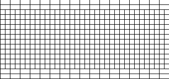
(Note the seeming absence of a border on the north and east. That’s intentional! Remember, we’re only drawing the west and south boundaries of each cell, because the entire thing wraps around. The grid’s western boundary is also its eastern boundary.)
Using POV-Ray, it’s straightforward to generate an image of this mapped onto a torus. Call the following file torus-map.pov:
#version 3.7;

global_settings {
  assumed_gamma 2.0
}

background { color rgb 1 }

light_source {
  <-50, 50, -50> color rgb <1, 1, 1>
}

camera {
  location <3, 8, -15>
  look_at  <0, -2, 0>
}

torus {
  1, 0.5
  texture {
    pigment {
      image_map {
        png "torus-grid.png"
        map_type 5
      }
    }
    finish { ambient 0.2 phong 0.5 }
  }
  scale 6
}
Assuming you have POV-Ray installed, you can generate the corresponding image like this. (The +A0.001 instructs POV-Ray to use some pretty intense anti-aliasing; otherwise, the lines of the maze will look terribly jaggy.)
$ povray torus-map.pov +A0.001
...
POV-Ray finished
The resulting image will be called torus-map.png. Check it out!
Let’s finish this off by taking the next logical step. We can easily generate a maze using the Recursive Backtracking algorithm:
stack = [ grid.sample ]

while stack.any?
  current = stack.last
  neighbor = current.neighbors.
    select { |n| n.links.empty? }.sample

  if neighbor
    current.link!(neighbor)
    stack.push(neighbor)
  else
    stack.pop
  end
end

grid.to_png.save("torus-maze.png")
If we then replace torus-grid.png with torus-maze.png in the POV-Ray input file, we get this:
Isn’t that lovely?
Mazes are fun. :)
(P.S. If you want to play around with this code without having to reconstruct it from the code snippets above, here’s a gist with the whole thing.)
